In this short guide you can learn the basics of linear regression in Python. Linear regression is a model which represents the relation of variables - they can be independent or dependent. Linear regression can help to answer the question of dependency or numeric variables.
So let's explain it in a simple example. Suppose you are a data scientist which is asked:
Is there a relation between money and happiness?
To prove it you will need to do it in several steps:
- define the question (it's already done)
- find data
- analyse it
- summarize it
Step 1: Find and prepare data for Linear Regression
Once the question is defined we can search for data. Then you may need to do some preprocessing of the data like:
- clean - bad records, incomplete data
- format issues
Suppose we have data like:
import pandas as pd
import numpy as np
import matplotlib as mpl
import matplotlib.pyplot as plt
from sklearn.linear_model import LinearRegression

# import and preview dataset
df = pd.read_csv("https://raw.githubusercontent.com/softhints/dataplotplus/master/data/happyscore_income.csv")
| country | adjusted_satisfaction | avg_income | happyScore |
|---|---|---|---|
| Armenia | 37.0 | 2096.76 | 4.350 |
| Angola | 26.0 | 1448.88 | 4.033 |
| Argentina | 60.0 | 7101.12 | 6.574 |
| Austria | 59.0 | 19457.04 | 7.200 |
| Australia | 65.0 | 19917.00 | 7.284 |
Data is taken from Kaggle and there's no need to clean or process it.
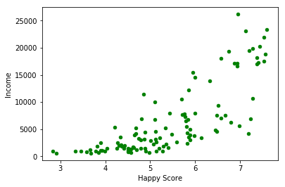
Step 2: Scatterplot and Linear Regression
In this step we are going to plot simple Scatterplot in Python. We need two numeric variables like:
# basic plot scatter
plt.xlabel('Happy Score')
plt.ylabel('Income')
plt.scatter('happyScore', 'avg_income', data=df, s=20, color='green')
result:
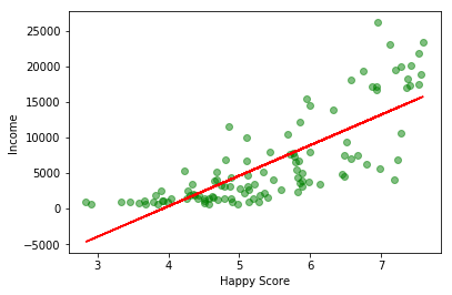
Next step is to perform the linear regression. We are going to search for the relation between happyScore and avg_income. We are using class: LinearRegression from sklearn.linear_model
X = df['happyScore'].values.reshape(-1, 1)
Y = df['avg_income'].values.reshape(-1, 1)

linear_regressor = LinearRegression()
linear_regressor.fit(X, Y)
Y_pred = linear_regressor.predict(X)
The result is array of predicted values like:
array([[ 1842.30538429],
       [  481.79795859],
       [11387.31647189],
       [14073.99675104],
       [14434.50975975],
       [ 5541.85554504],
       [ 3318.69199137],
Step 3: Plot Linear Regression in Python
Finally we are going to** plot the regression line on the scatterplot** from the previous step:
plt.xlabel('Happy Score')
plt.ylabel('Income')

plt.scatter(X, Y, color='green', alpha=0.5)
plt.plot(X, Y_pred, color='red')
plt.show()
the result shows that there might be a relation between those two:
Step 4: Polynomial Linear Regression in Python
Finally let's check how to extend linear regression with polynomial features in Python. This approach is more precise in some cases:
from sklearn.preprocessing import PolynomialFeatures

# prepare Polynomial Features
pr = PolynomialFeatures(degree = 5)
X_poly = pr.fit_transform(X)
pr.fit(X_poly, Y)

# Polynomial Linear Regression
lin_reg = LinearRegression()
lin_reg.fit(X_poly, Y)

# plot
plt.scatter(X, Y, color='green', alpha=0.5)
plt.scatter(X, lin_reg.predict(pr.fit_transform(X)))
plt.show()
The result:
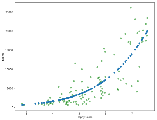
We are fitting the model with degree = 5 which:
- degree equal to 1 will be the same as the linear regression
- higher degree will take more time to compute
- higher degree will match relation better
Example for degree 15: